Too much data in a single column can make your MS Excel spreadsheet generally harder to read. In order to improve it, you should consider splitting up your column using the “Text to Columns” or “Flash Fill” features. Here’s how to Make One Long Column into Multiple Columns in MS Excel.

“Text to Columns” will basically replace your single column with multiple columns using the same data. “Flash Fill” will generally replicate the data, splitting it into new, individual columns while leaving the original column intact.
How to Use Text to Columns in MS Excel
MS Excel includes a special feature which allows you to split up extra long columns. It does this by separating columns using delimiters, such as commas or semicolons, which split up the data.
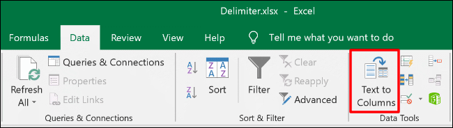
This feature works by using Text to Columns, which you can access from the “Data” tab in your Microsoft Excel ribbon bar.
For testing this feature, we’ll be using a set of data (an employee list, showing names, dates of birth, and other information) in a single column. Each section of data is in a single cell is separated by a semicolon.
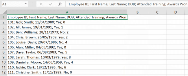
You’ll need to select the cells containing your data first cells A1 to A12 in the example above.
Then from Excel’s “Data” tab, tap on the “Text to Columns” button found in the “Data Tools” section.
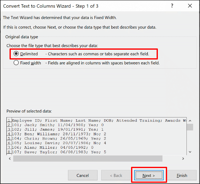
This will bring up the “Convert Text to Columns Wizard” window and will allow you to begin separating your data. From the options, select the “Delimited” radio button and tap on “Next” to continue.
Excel will choose to try and separate your single column data by each tab it finds by default. This is fine, however for our example, we are using data that are separated by semicolons only.
Select your delimiter option from the side menu. For our example, our chosen delimiter is a semicolon.

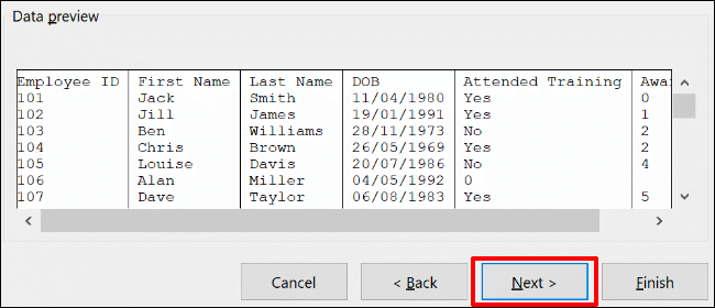
Now you can see how the converted data will look in the “Data Preview” section at the bottom of the menu.
Once you’re ready, tap on “Next” to continue.
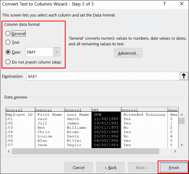
Now you will need to set the cell types for each column. For example, if you have a column with dates, you can set the appropriate date format for that column. By default, each column will be set to the “General” setting.
Using this option, Excel will attempt to set the data type for each column automatically. To set these manually, tap on your column in the “Data Preview” section first. From there, choose the appropriate data type from the “Column Data Format” section.
In case you want to skip a column completely, select your column, then select the “Do Not Import Column (Skip)” option. Tap on “Finish” to begin the conversion.
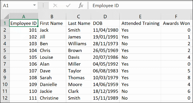
Your single column will separate each section by using the delimiters, into individual columns using the cell formatting options you selected.
How to Use Flash Fill in Excel
In case you’d like to keep your original data intact, however still separate the data, you can use the “Flash Fill” feature instead.
Using our employee list example, we have a single column (column A) header row, with a semicolon delimiter separating each bit of data.

In order to use the “Flash Fill” feature, start by typing out the column headers in row 1. For our example, “Employee ID” would go in cell B1, “First Name” in cell C1, etc.
For each column, select your header row. Start with B1, the “Employee ID” header in this example and then, in the “Data Tools” section of the “Data” tab, tap on the “Flash Fill” button.

Now repeat the action for each of your header cells (C1, D1, etc) to automatically fill the new columns with the matching data.
If the data is formatted correctly in your original column then Excel will automatically separate the content using the original header cell (A1) as its guide.
In case you receive an error, then type the following value in the sequence in the cell below your header cell and then click the “Flash Fill” button again.
According to our example, that would be the first data example in cell B2 “101” after the header cell in B1 “Employee ID”.
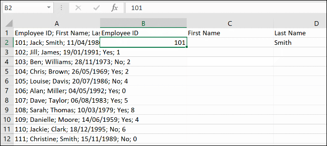
Each new column will fill with the data from the original column by using the initial first or second rows as the guide to choose the correct data.
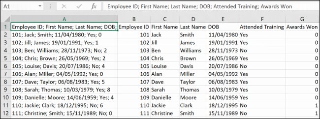
In the example above, the long column – column A separates into six new columns B to G.
Due to the layout of rows, 1 to 12 is the same, the “Flash Fill” feature is able to copy and separate the data, using the header row and first bit of data.